Divididend analysis of Telenor ASA using Jupyter Notebook

Cross posted from Divididend analysis of Telenor ASA using Jupyter Notebook

I just published the notebook dividends.ipynb on my GitHub repository jorisp/tradingnotebooks which shows how dividends contribute to the total return. This notebook uses the yfinance API to retrieve the data.  I used Telenor ASA (a Norwegian telecom operator) as an example.

If you are considering to invest in foreign dividend stocks as a Belgian investor, you need to keep in mind the double taxation of dividends. Even with a withholding tax applied abroad, the Belgian government will tax your dividend again at a flat rate of 30%.

Disclaimer: The information on this blog is intended solely for informational and educational purposes. I am not a certified financial advisor, and the content provided here does not constitute professional financial advice. (Full disclaimer)

Getting financial data in Python using the OpenBB SDK

The OpenBB SDK (also known as OpenBB Platform) is developed as open-source (the code is available on https://github.com/OpenBB-finance/OpenBB) by the company Open BB. The OpenBB SDK provides programmatic access to a wide range of financial data sources from one place in a standard way.

The OpenBB SDK was developed to drive the OpenBB Workspace (See Introducing the new OpenBB Terminal ) which provides a customizable platform for financial analysts, investors and researchers that rivals traditional financial terminals without the steep costs.

By default, the OpenBB SDKwill attempt to download data from free sources such as Yahoo Finance but OpenBB SDK integrates with multiple other data sources as well such as , Alpha Vantage, FRED,FMP,SEC,etc .... In most OpenBB API platform calls, you can indicate a different data source - some of them free others requiring a separate subscription - allowing you to pull equities, options, crypto, forex and macroeconomic data using a single SDK. 

Since you can access both historical and real-time market data, OpenBB is ideal for backtesting and live trading strategies. The SDK is compatible with Jupyter Notebooks, Python scripts, and automated trading systems. I recently tested the OpenBB SDK as an alternative to Pandas_DataReader in Jupyter Notebooks, and it worked flawlessly.

I shared this Jupyter notebook on my Github repo:

https://github.com/jorisp/tradingnotebooks/blob/master/openbbdemo.ipynb

Please note that many of the code samples found in various articles and posts are no longer functional due to significant changes in the codebase. The shared Jupyter notebook has been tested with OpenBB 4.3.5 and Python 3.12.8.

The Rational Reminder podcast - favorite episodes from 2024

I started listening to the Rational Reminder Podcast somewhere around the beginning of this year and I can highly recommend it to anyone interested in passive evidence based investing and financial decision making. 

The Rational Reminder podcast is weekly podcast about personal finance and investing from a couple of Canadians, Benjamin Felix and Cameron Passmore - both work at PWL Capital. The hosts are experienced portfolio managers who share their knowledge about a broad range of financial topics and the show often features interviews with industry experts, offering diverse perspectives and deep dives into specific areas of finance.

Benjamin Felix also creates educational content on YouTube https://www.youtube.com/@BenFelixCSI where he shares insights on investing and financial planning

Both advocate for evidence-based investing, which often includes passive investment strategies such as index funds and they emphasize the benefits of low-cost, diversified, and long-term investment approaches, which align well with passive investing principles.

Episodes which I really liked:

• Episode 321 - Evidence in Practice with Håkon Kavli (CIO of Reitan Kapital)
• Episode 320 - Kyla Scanlon: In This Economy?!
• Episode 316 - Andrew Chen: "Is everything I was taught about cross-sectional asset pricing wrong?!" about Open Source Asset Pricing
• Episode 313 - When Should You Hire a Financial Advisor?
• Episode 310 - Professor Antoinette Schoar: Consumer Finance, Crypto, and Private Equity
• Episode 303 - Scott Galloway: The Algebra of Wealth
• Episode 302 - Michael Green: Market Efficiency Is Not The Question
• Episode 292 - Rob Copeland: Ray Dalio and Bridgewater
• Episode 291 - The Quant Winter, and is Canada Pension Plan a Scam?
• Episode 289 - Retiring Retirement Income Myths with the Retirement Income Dream Team
• Episode 286: Errol Morris: Tuning out the Noise

Book review: beyond diversification - what every investor needs to know about asset allocation

I recently finished reading Beyond diversification from Sebastien Page.  Sebastien Page (Chief Investment Officer at T. Rowe Price) explains in Beyond diversification the different approaches to forecasting returns, risks and correlations across asset classes by combining academic research and practical hands-on examples. 

This book is most likely targeted at the sophisticated investor  and should not be the first book to pick up if you want to understand diversification but it provides great insights on how asset managers think about their portfolios. 

The book also extensively refers to a number of academic papers that Sebastien Page has written on asset allocation, risk measurement and return forecasting. It explores a number of dynamic asset allocation strategies, acknowledging that risk is time-varying and requires adaptive approaches. Sebastien Page also explains why the typical fixed weight asset allocation (60-40 portfolio) does not deliver a constant risk exposure.

The book recommends using a  heuristics to cope with changes in volatility: assume that next month's volatility for each asset class will be the same as last month's. For the longer term the opposite is true, 5 years of calm markets are more likely to be followed by 5 years of turbulence.

The stock-bond mix is the biggest decision that multi-asset investeros make, but this mix does not reliably reduce risk as correlations shift. Stock bond correlations were positive in the 1970s and 1980s when inflation and interest rates drove volality but then the correlation reversed.

PS With volatility being a proxy for risk, you might also check out the white paper "Practical Issues in Forecasting volatility" from Clive Granger and Ser Huang Poon which was published in the Financial Analyst Journal in February 2005.

Looking at historical returns of stocks and bonds with Power BI and Python

You might already have seen below graph taken from a study by JP Morgan Asset Management, but what if you would like to look at historical returns without going  through the hassle of having to collect all the data yourself?

There is an interesting Excel sheet shared by Aswath Damodaran (@AswathDamodaran)  that you can download from Historical Returns on Stocks, Bonds and Bills: 1928-2022 which looks at returns of different asset classes (stocks, bonds, bills, real estate and gold) over a longer time period.

In this post I will share some tips on how you can use this data in Power BI, Python and Jupyter notebooks. 

This Historical Returns on Stocks, Bonds and Bills: 1928-2023 - Excel file  file is updated in the first two weeks of every year and it is being maintained by Aswath Damodaran, who is a professor of Finance at the Stern School of Business at NYU, he is also known as the "Dean of Valuation" due to his experience in this area.

Visualizing S&P 500 and US Treasury bond returns using Power BI

I first converted the Excel from  xls to xlsx format and afterwards it is quite easy to  import the data from an Excel workbook files in Power BI . It is quite easy to visualize the returns of  both stocks and US treasury bonds using a clustered column chart - I also added a minimum line for both stock and bond returns.

Expected risk and expected return should go hand in hand: the higher the expected return, the higher the expected risk. Risk means means that the future actual return may vary from the expected return (and the ultimate risk is loosing all of your assets). The first visual showed a 20-year annualized return between 1999 and 2018 for the S&P 500 of 5.8%.  Average returns hide however the big swings in yearly returns - e.g. in 2008 (the Great Financial Crisis), the S&P 500 had a -36.5% yearly return. Bonds on average have a lower return but also have a lower risk profile. 

The basic rule of thumb is to keep your “safe money” (i.e., money you don’t want to risk in stocks) in high-quality bonds. While this doesn’t give you 100% protection against losses at all times, it does provide you some peace of mind. I really like this quote: "If you can't sleep at night because of your stock market position, then you have gone too far. If this is the case, then sell your positions down to the sleeping level. (Jesse Livermoore)"

As you can see in the visualization below, in most years with a negative return for the S&P 500, the return for bonds is positive - with two notable exceptions 1969 and 2022. A common saying is to have your age in bonds. Using that general rule, a 45-year-old might have 45% of the total portfolio in bonds. If you want to more aggressive, you would have less than your age in bonds. The last decade with interest rates very low (or even negative) this probably wasn't a very profitable asset allocation but 

things might have shifted.

The US Treasury Bond used in the Excel file is the 10-year US treasury bond for which you can download the data from FRED . The yearly return has been calculated by taking the yield and the price change for a par bond with that specific yield.

You can download the Power BI file histreturns.pbix from my Power BI Github repo

In the long run (see example below for different rolling windows from a 1-year to a  20 year period)  stocks will outperform bonds but this again works with averages and it ignores the tail risk which might wreak havoc in your portfolio.

Reading data from Excel using Python

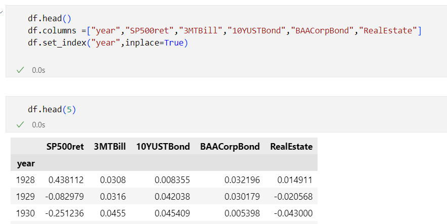
Now let's take a look at how you can read and manipulate the data in this Excel sheet using Python. To read an excel file as a DataFrame, I will use the pandas read_excel() method. Internally, Pandas. .read_excel uses a library called xlrd which you also need to install but I used the  openpyxl library as an alternative which also works. So before you can read an excel file in pandas, you will need to install 

the openpyxl library. 

The above code reads only the table with data from the Excel file (which I downloaded in a subdirectory data from the Jupyter notebook) - see  pandas.read_excel in the Pandas referencel documentation for full details:

• sheet_name: can be an integer (for the index of a worksheet in an Excel file, default to 0, the first sheet) or the name of the worksheet you want to load
• nrows: number of rows to read
• skiprows: number of rows to skip
• usecols: by default all columns will be read but also possible to pass in a list of columns to read into the dataframe like in the example

I just started exploring some data around stock-bond correlations and will be updating the Juypyter notebook on Github - https://github.com/jorisp/tradingnotebooks/blob/master/HistoricalReturns.ipynb

A couple of weeks ago I noticed this interesting tweet on rolling one-year-stock-bond correlations for six regimes from @WifeyAlpha - I think it would make an interesting exercise to see how to rebuild this using Python.

References:

• Pandas – read_excel() – How to read Excel file in python
• Musings on markets: a return to teaching - the Spring 2023 Edition
• Guide to the Markets | JP Morgan Asset Management

Related posts:

• Interactive chart visualizations using Python and bqplot: visualizing S&P500 returns
• Using the yFinance Python package to download financial data from Yahoo Finance - part 2
• Using the yFinance Python package to download financial data from Yahoo Finance
• Using Python and Pandas Datareader to retrieve financial data - part 2: Fama & French data library
• Using Python and Pandas Datareader to retrieve financial data - part 1: Federal Reserve Data (FRED)

Interactive chart visualizations using Python and bqplot: visualizing S&P500 returns

A couple of months ago, I stumbled upon this interesting presentation Jupyter Notebooks: interactive visualization approaches. The presentation showed how you can use bqplot to build interactive visualizations. 

Bqplot contains a set of 2D plotting widgets built on top of the ipywidgets framework for Jupyter notebooks. The bqplot package aims to bring d3.js visualizations to Python while retaining the flexibility and ease of use of ipywidgets and was developed by the quantitative research team at Bloomberg. You can install bqplot using conda or pip. 

One of the examples built by the team that you can find on Github is a Jupyter notebook which shows US equity market performance (using the S&P 500 index) where you can select an interval on a time series chart - for the selected area you get the total return as well as a histogram of the daily returns.

References:

• Interactive data visualization using Bqplot
• bqplot - Interactive plotting in Jupyter notebook
• bqplot: bringing more interactivity to data

Visualize S&P 500 data in Power BI using Azure Synapse Serverless SQL Pool

In Explore and analyze stock ticker data in Azure data lake with Azure Synapse serverless SQL Pool, I showed you can download stock ticker data from Yahoo Finance, stored it in Azure Data Lake and retrieve the data using standard T-SQL in Azure Synapse Studio. In this post, I will show how easy it is to consume the data from Synapse SQL Serverless using Power BI.

For the standard visual with the evolution of the S&P 500 closing price, I connected directly on SP500 external table in the Synapse SQL. You can connect to Synapse SQL Serverless using either the Azure SQL Database or Azure Synapse Analytics SQL connector and you will need to enter the Serverless SQL endpoint which looks something like this <yoursynapse>-ondemand.sql.azuresynapse.net

With the second reported I want to visualize the S&P 500 yearly return and the average return since December 1927. To make it easier, I created a separate view on top of the external table which calculates the yearly returns

As you see from the visual, returns can vary quite a lot both on the negative side as well as on the positive side - for the last 20 years, there was a huge drop in 2008 (-38%) and also this year is not looking great (-22%), but 2013, 2019 and 2021 all had returns above 20%. On average across the S&P 500 returned 7% (not included dividends).

For the last visual in the Power BI report, I wanted to show a histogram with the S&P 500 yearly returns. I based myself on Power BI Histogram example using DAX since  Power BI does not have a standard histogram and I did not want to use a custom visual ( I used Power BI custom visuals from Pragmatic Works in the past)

Equity returns roughly follow a normal distribution or "bell curve", meaning that most values cluster near the central peak and values farther from the average are less common.  Stock returns however have fat tails - meaning that the occurrences on the extremes are far more common than expected in a normal distribution.  The Greate Depression (1931) and the Global Financial Crisis (2008) led to two of the largest stock market losses of the S&P 500. With a loss between -20% and -30% this year, we are in the same category/bin as 1930, 1974 and 2002.

You can download the synapsestockdemo.pbix file and the benchmark.csv file from my Power BI repo on GitHub

References:

• Tutorial: Use serverless SQL pool with Power BI  Desktop & create a report
• Tutorial: Explore and analyze data lakes with serverless SQL pool
• Power BI connectors to Azure Synapse

Using the yFinance Python package to download financial data from Yahoo Finance - part 2

In a previous post I showed how you can download ticker data from Yahoo Finance using the yFinance Python package.  I now updated the  Jupyter notebook code sample using YFinance to also show how you can retrieve additional information (sector, industry, trailing and forward earnings per share, etc...). The Ticker class in the yFinance library contains the info property which returns a dictionary object ( a collection of key-value pairs where each key is associated with a value) which allows you to access specific information about an asset.

Since I wanted to know how fast data retrieval would be I also include the %%time magic command . Wall clock time measures how much time has passed. CPU time is how many (milli)seconds the CPU was busy.

Yahoo Finance contains data about stocks, Exchange Traded Funds  (ETF), mutual funds and stock market indices - the information that you can retrieve for each of these differs, so it is safe to check in your code for the quoteType. Below example retrieves information about Apple stock, the iShares MSCI AWCI UCITS ETF (Acc) and a thematic mutual fund from KBC.

I also included a code snippet which shows how to retrieve this information for multiple assets and convert this into a Pandas dataframe.

Using the yFinance Python package to download financial data from Yahoo Finance

In a previous post I explained how you can retrieve data from Yahoo Finance using Python and Pandas Datareader - an alternative Python library for retrieving data from Yahoo Finance is yFinance maintained by Ran Aroussi. 

If you are using conda package manager, you will notice that you can not install yfinance using conda so you will need to revert to pip install yfinance. All documentation is available on yFinance  as well as on https://github.com/ranaroussi/yfinance but I also uploaded a  Jupyter notebook code sample on my Github - https://github.com/jorisp/tradingnotebooks/blob/master/yfinance_sample.ipynb

Using Python and Pandas Datareader to retrieve financial data - part 2: Fama & French data library

This post is part of a series on using Pandas datareader to retrieve financial data:

• Using Python and Pandas Datareader to retrieve financial data - part 1: Federal Reserve Data (FRED)
• Using Python and Pandas Datareader to retrieve financial data - part 2: Fama & French library
• Using Python and Pandas Datareader to retrieve financial data - part 3: Yahoo Finance

In this post we will look at the datasets made available by Eugene Fama and Kenneth French. Eugene Fama and Kenneth French did a lot of research on which factors drive security returns. In 1993, they published the Three Factor Model (see article "Common risk factors in returns of stocks and bonds", Journal of Financial Economics 33, 1993), which showed that their factors (size of the firm, book-to-market values and excess return) capture a statistically significant fraction of the variation of stock returns. In 2014, Fama and French adapted their model to include five factors.  Fama won the Nobel Prize for Economics in 2013 for his research. Fama also published a number of papers on the Efficient Market Hypothesis and random walk theory.

Fama and French still publish the returns of various investment factors analyzed by them on their homepage on a regular basis.  You can download this data using the pandas_datareader library - you can take a look at the official documentation,  Fama-French Data (Ken French's Data library) to get started or take a look at the Jupyter notebook that I shared on Github https://github.com/jorisp/tradingnotebooks/blob/master/FAMA.ipynb

References:

• Fama/French forum ideas and observations from Fama and French
• How to use the Fama French model
• Fama-French 5-factor model: five major concerns
• In pursuit of the perfect portfolio: Eugene F. Fama (YouTube - MIT Laboratory for Financial Engineering )

Palm oil price vs SIPEF stock price in Jupyter notebooks with Quandl

Quandl also offers free commodity price data for almost 100 commodities ( See API for commodity data) so I decided to create a Jupyter notebook comparing SIPEF's stock price with the price of palm oil. Take a look at the full notebook I shared on github if you want to learn why - https://github.com/jorisp/tradingnotebooks/blob/master/Quandl_API_Euronext_SIPEFPalmOil.ipynb 

 

Remarks:

• Be careful when embedding images in a Jupyter notebook that you want to publish on Github (see Images in Markdown not showing when uploaded to Git for a discussion on this) - filenames are case sensitive - I got it working using the url syntax
• To store the quandl key I used the approach outlined on how to use secrets in Jupyter Notebooks with python-dotenv
• I really like Matplotlib and its versatility in rendering capabilities  in this notebook I used the ability to visualize multiple time series (see code preview below) with different axes. (see code below)

sipcolor = 'tab:red'
fig,ax1 = plt.subplots()

ax1.plot(data['SIP'],color=sipcolor)
ax1.set_ylabel('SIPEF',color=sipcolor)
#Instantiate a second axes that shares the same x-axis
ax2 = ax1.twinx()
ax2.plot(data['PPOIL'])
ax2.set_ylabel('PALM OIL USD')
plt.gcf().set_size_inches(15,8)
plt.show()

Related posts:

• Working with multiple time series trading data from Quandl in Jupyter Notebooks
• Using Euronext  stock data from Quandl in Jupyter Notebooks

Working with multiple time series trading data from Quandl in Jupyter Notebooks

In the previous example - Using Euronext stock data from Quandl in Jupyter notebooks I downloaded a single dataset from Quandl. But it is also possible to download multiple datasets by passing in a list of Quandl codes.

In the example below, I downloaded the prices of a number of diversified holding companies which are traded on Euronext Brussels and compared the cumulative returns (not including dividend payments) using Jupyter Notebooks.

The Quandl Python API allows you to make a filtered time series call and request only specific
columns - in this example the 'Last' (Closing price) is retrieved by specifying the index 4. In a next
step I renamed the columns in the pandas dataframe to make it easier to work with the data
afterwards.



Take a look at the full python notebook at https://github.com/jorisp/tradingnotebooks/blob/master/Quandl_Belgian_Holdings-Shared.ipynb to see how this data can be used to visualize cumulative returns for these different stocks

1 2 3 4 5 6 7 8 9 10 11 12 13 14 15

%matplotlib inline import quandl import matplotlib.pyplot as plt quandl.ApiConfig.api_key = "<Your Key Here>" #Retrieve Last price only for the 5 holdings (excluding mono holdings) trading on Euronext Brussels #Data is available from February 2014 onwards - Ackermans Van Haren (ACKB), Brederode (BREB), Sofina (SOF), #GBL and Bois Sauvage (COMB ) data = quandl.get(['EURONEXT/ACKB.4','EURONEXT/BREB.4','EURONEXT/SOF.4','EURONEXT/GBLB.4','EURONEXT/COMB.4']) #Rename column names data.rename(columns={'EURONEXT/ACKB - Last': 'ACKB', 'EURONEXT/BREB - Last': 'BREB','EURONEXT/SOF - Last':'SOF', 'EURONEXT/GBLB - Last':'GBLB','EURONEXT/COMB - Last':'COMB'},inplace=True)

Using Euronext stock data from Quandl in Jupyter notebooks

The last couple of weeks I have been learning about Python and how to use it for stock and derivative trading. One of the challenges is getting stock trading data for European stocks (without having to pay for it).  One of the first things I started with is using Jupyter notebooks to quickly visualize stock market information.

The easiest way to get started with Jupyter is using an all-in-one Python distribution - the one I used is Anaconda since it is easy to setup and it includes a number of interesting libraries I want to use in next steps.

I like to try out things hands-on but I did use a number of training resources to get up to speed:

• Jupyter Notebook Tutorial: the definitive guide (Datacamp)
• Create and share Analytics with Jupyter Notebooks (Pluralsight) 

To get trading data about European stocks I used Quandl. Quandl is a marketplace for financial and economic data which is either freely available or requires a paid subscription. Data is contributed by multiple data publishers like World Bank, trading exchanges and investment research firms. Quandl provides REST API access to the available data sets but also has specific Python and R libraries. You first need to register to get an API key. A lot of European stocks are traded on Euronext and Quandl provides you access to Euronext data - https://www.quandl.com/data/EURONEXT-Euronext-Stock-Exchange

Install the quandl Python package using the Anaconda command prompt. It is best to setup virtual environments to manage separate package installation that you need for a particular project, isolating the packages in other environments but for simplicity I just installed in the base environment.

Next it is quite easy to retrieve stock data from Quandl - you first import the quandl package and next you call the quandl.get() method. By default, Quandl will retrieve the dataset into a pandas DataFrame. Since I specified no additional parameters, the entire timeseries dataset was retrieved - from February 2014 until now. Afterwards I used the plot command which uses the matplotlib library to display a graph of the closing prices.

For the full Jupyter notebook take a look at Github https://github.com/jorisp/tradingnotebooks/blob/master/Quandl_API_Euronext_ABI_Shared.ipynb

References:

Wednesday, November 16, 2022
Thursday, September 03, 2020