Quick tip: how to check the Python version and packages installed in a Python virtual environment

 Activate the environment and run python --version or python -V

To check a specific package e.g. streamlit run pip show streamlit inside the anaconda prompt

Understanding conda channels

 Conda channels are package source - locations where conda looks for software packages when you run conda install. Each channel can contain different package versions, build configurations, platform-specific binaries, etc ...

In the screenshot above, you will notice 4 different conda channels:

• defaults: the official Anaconda repository, has stable, curated with conservative updates
• microsoft: Microsoft maintains its own channel mainly for AzureML environment support or packages tuned for Windows performance.
• anaconda: similar to the defaults channel
• conda-forge: community driven, massive ecosystem with the latest versions. Receives updates within hours of upstream releases

You can add a channel using this command: conda config --add channels microsoft. Conda searches channels in order, from highest priority to lowest. So from my configuration, it first try to install from defaults. If not found, it falls back to microsoft, and so on ...

Quick tip: retrieving raw, unprocessed files stored in Github

 The domain raw.githubusercontent.com serves raw, unprocessed files stored in Github repositories - think of it as GitHub's "direct file download" backend. Tools like curl, wget or Python scripts can fetch files directly using a specific url composed of the user name, repo, branch, folder and filename

curl -O https://raw.githubusercontent.com/[user]/[repo]/[branch]/[folder]/[filename] 

example: curl -O https://raw.githubusercontent.com/jorisp/tradingnotebooks/master/data/DJI.csv

You can also read these raw files form GitHub using pandas.read_csv

Interactive Pandas dataframes with ITables 2.0

 ITables is a Python package available on Github (maintained by Marc Wouts) which changes how Pandas and Polars dataframes are rendered in Python notebooks and other Python applications. It works out of the box without any dependencies in Jupyter, Dash, Streamlit and Marimo. 

For more info see:

• Make your Pandas or Polars DataFrames Interactive with ITables 2.0
• ITables Quick Start

Enable and disable Data Wranger in VS Code for Pandas DataFrame and Series

To disable default rendering of Pandas DataFrames in VS Code Jupyter Notebook with Data Wrangler (after installing the extension) - follow these steps:

1. Open Command Palette : Preferences: Open Settings (UI)
2. Search for: Data Wrangler
3. Uncheck the Data Wrangler>Output Renderer: Enabled Types for Pandas Dataframe and Series to disable the rendering and check them again when needed

Related links:

• Getting started with Data Wrangler in VS Code

Divididend analysis of Telenor ASA using Jupyter Notebook

Cross posted from Divididend analysis of Telenor ASA using Jupyter Notebook

I just published the notebook dividends.ipynb on my GitHub repository jorisp/tradingnotebooks which shows how dividends contribute to the total return. This notebook uses the yfinance API to retrieve the data.  I used Telenor ASA (a Norwegian telecom operator) as an example.

If you are considering to invest in foreign dividend stocks as a Belgian investor, you need to keep in mind the double taxation of dividends. Even with a withholding tax applied abroad, the Belgian government will tax your dividend again at a flat rate of 30%.

Disclaimer: The information on this blog is intended solely for informational and educational purposes. I am not a certified financial advisor, and the content provided here does not constitute professional financial advice. (Full disclaimer)

Getting financial data in Python using the OpenBB SDK

The OpenBB SDK (also known as OpenBB Platform) is developed as open-source (the code is available on https://github.com/OpenBB-finance/OpenBB) by the company Open BB. The OpenBB SDK provides programmatic access to a wide range of financial data sources from one place in a standard way.

The OpenBB SDK was developed to drive the OpenBB Workspace (See Introducing the new OpenBB Terminal ) which provides a customizable platform for financial analysts, investors and researchers that rivals traditional financial terminals without the steep costs.

By default, the OpenBB SDKwill attempt to download data from free sources such as Yahoo Finance but OpenBB SDK integrates with multiple other data sources as well such as , Alpha Vantage, FRED,FMP,SEC,etc .... In most OpenBB API platform calls, you can indicate a different data source - some of them free others requiring a separate subscription - allowing you to pull equities, options, crypto, forex and macroeconomic data using a single SDK. 

Since you can access both historical and real-time market data, OpenBB is ideal for backtesting and live trading strategies. The SDK is compatible with Jupyter Notebooks, Python scripts, and automated trading systems. I recently tested the OpenBB SDK as an alternative to Pandas_DataReader in Jupyter Notebooks, and it worked flawlessly.

I shared this Jupyter notebook on my Github repo:

https://github.com/jorisp/tradingnotebooks/blob/master/openbbdemo.ipynb

Please note that many of the code samples found in various articles and posts are no longer functional due to significant changes in the codebase. The shared Jupyter notebook has been tested with OpenBB 4.3.5 and Python 3.12.8.

Quick note: Python date and time objects

In Python, a naive datetime object is one that does not contain any information about time zones or daylight saving time. This means it is unaware of the context in which it exists, such as whether it represents local time, UTC, or any other time zone. By default, the datetime object in Python is naive. You can make them timezone aware using the pytz library.

If you are working with pandas dataframes or series, you can also use the tz_localize method of the Pandas DateTimeIndex object.

References:

•  datetime - basic date and time (Python docs)
• pandas.Series.tz_localize

Looking at historical returns of stocks and bonds with Power BI and Python

You might already have seen below graph taken from a study by JP Morgan Asset Management, but what if you would like to look at historical returns without going  through the hassle of having to collect all the data yourself?

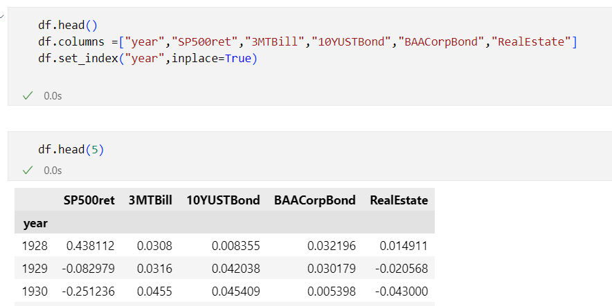
There is an interesting Excel sheet shared by Aswath Damodaran (@AswathDamodaran)  that you can download from Historical Returns on Stocks, Bonds and Bills: 1928-2022 which looks at returns of different asset classes (stocks, bonds, bills, real estate and gold) over a longer time period.

In this post I will share some tips on how you can use this data in Power BI, Python and Jupyter notebooks. 

This Historical Returns on Stocks, Bonds and Bills: 1928-2023 - Excel file  file is updated in the first two weeks of every year and it is being maintained by Aswath Damodaran, who is a professor of Finance at the Stern School of Business at NYU, he is also known as the "Dean of Valuation" due to his experience in this area.

Visualizing S&P 500 and US Treasury bond returns using Power BI

I first converted the Excel from  xls to xlsx format and afterwards it is quite easy to  import the data from an Excel workbook files in Power BI . It is quite easy to visualize the returns of  both stocks and US treasury bonds using a clustered column chart - I also added a minimum line for both stock and bond returns.

Expected risk and expected return should go hand in hand: the higher the expected return, the higher the expected risk. Risk means means that the future actual return may vary from the expected return (and the ultimate risk is loosing all of your assets). The first visual showed a 20-year annualized return between 1999 and 2018 for the S&P 500 of 5.8%.  Average returns hide however the big swings in yearly returns - e.g. in 2008 (the Great Financial Crisis), the S&P 500 had a -36.5% yearly return. Bonds on average have a lower return but also have a lower risk profile. 

The basic rule of thumb is to keep your “safe money” (i.e., money you don’t want to risk in stocks) in high-quality bonds. While this doesn’t give you 100% protection against losses at all times, it does provide you some peace of mind. I really like this quote: "If you can't sleep at night because of your stock market position, then you have gone too far. If this is the case, then sell your positions down to the sleeping level. (Jesse Livermoore)"

As you can see in the visualization below, in most years with a negative return for the S&P 500, the return for bonds is positive - with two notable exceptions 1969 and 2022. A common saying is to have your age in bonds. Using that general rule, a 45-year-old might have 45% of the total portfolio in bonds. If you want to more aggressive, you would have less than your age in bonds. The last decade with interest rates very low (or even negative) this probably wasn't a very profitable asset allocation but 

things might have shifted.

The US Treasury Bond used in the Excel file is the 10-year US treasury bond for which you can download the data from FRED . The yearly return has been calculated by taking the yield and the price change for a par bond with that specific yield.

You can download the Power BI file histreturns.pbix from my Power BI Github repo

In the long run (see example below for different rolling windows from a 1-year to a  20 year period)  stocks will outperform bonds but this again works with averages and it ignores the tail risk which might wreak havoc in your portfolio.

Reading data from Excel using Python

Now let's take a look at how you can read and manipulate the data in this Excel sheet using Python. To read an excel file as a DataFrame, I will use the pandas read_excel() method. Internally, Pandas. .read_excel uses a library called xlrd which you also need to install but I used the  openpyxl library as an alternative which also works. So before you can read an excel file in pandas, you will need to install 

the openpyxl library. 

The above code reads only the table with data from the Excel file (which I downloaded in a subdirectory data from the Jupyter notebook) - see  pandas.read_excel in the Pandas referencel documentation for full details:

• sheet_name: can be an integer (for the index of a worksheet in an Excel file, default to 0, the first sheet) or the name of the worksheet you want to load
• nrows: number of rows to read
• skiprows: number of rows to skip
• usecols: by default all columns will be read but also possible to pass in a list of columns to read into the dataframe like in the example

I just started exploring some data around stock-bond correlations and will be updating the Juypyter notebook on Github - https://github.com/jorisp/tradingnotebooks/blob/master/HistoricalReturns.ipynb

A couple of weeks ago I noticed this interesting tweet on rolling one-year-stock-bond correlations for six regimes from @WifeyAlpha - I think it would make an interesting exercise to see how to rebuild this using Python.

References:

• Pandas – read_excel() – How to read Excel file in python
• Musings on markets: a return to teaching - the Spring 2023 Edition
• Guide to the Markets | JP Morgan Asset Management

Related posts:

• Interactive chart visualizations using Python and bqplot: visualizing S&P500 returns
• Using the yFinance Python package to download financial data from Yahoo Finance - part 2
• Using the yFinance Python package to download financial data from Yahoo Finance
• Using Python and Pandas Datareader to retrieve financial data - part 2: Fama & French data library
• Using Python and Pandas Datareader to retrieve financial data - part 1: Federal Reserve Data (FRED)

Interactive chart visualizations using Python and bqplot: visualizing S&P500 returns

A couple of months ago, I stumbled upon this interesting presentation Jupyter Notebooks: interactive visualization approaches. The presentation showed how you can use bqplot to build interactive visualizations. 

Bqplot contains a set of 2D plotting widgets built on top of the ipywidgets framework for Jupyter notebooks. The bqplot package aims to bring d3.js visualizations to Python while retaining the flexibility and ease of use of ipywidgets and was developed by the quantitative research team at Bloomberg. You can install bqplot using conda or pip. 

One of the examples built by the team that you can find on Github is a Jupyter notebook which shows US equity market performance (using the S&P 500 index) where you can select an interval on a time series chart - for the selected area you get the total return as well as a histogram of the daily returns.

References:

• Interactive data visualization using Bqplot
• bqplot - Interactive plotting in Jupyter notebook
• bqplot: bringing more interactivity to data

Notes on deploying and troubleshooting a Streamlit app on Azure App Services

 A couple of weeks ago I was playing around with Streamlit and decided to deploy it on Azure a
using Azure App Services using the guidance from Deploying Streamlit Applications with Azure App Services . 

Streamlit is an open-source Python library that allows you to create interactive, data-driven web applications in just a few lines of Python code. It does not require you to have any JavaScript, html or CSS experience.  

The deployment using the steps outlined in the blog post went quite smooth but when I navigated to the website, I was greeted by an exception.

Since I haven't worked with Linux for over 20 years now, I feared to be in for a long and painful experience to get this resolved but it actually turned out to be easier then expected. 

First step, I took was looking at the Application Logs for the Azure Web App. Go to the Azure App Service > Diagnose and solve problems > Application Logs. 

When scrolling through the Application Logs

The exception log "TypeError: Descriptor cannot be created directly. Your  generated code is 

out of data and must be regenerated with protoc > 3.19.0. If you cannot immediately

regenerate your protos, some other possible workarounds are: 1. Downgrade the protobuf package to 3.20.x or lower" actually pointed me to a thread on the Streamlit forums - Issue with Protocol Buffers. After changing requirements.txt  to deploy a newer version of Streamlit (see Configure a Linux Python App for Azure App Service for more details on how the Azure App Service deployment engine automatically runs pip install.) all started working correctly again.

References:

• Viewing Azure App Service web server and application logs in real time on Azure Portal
• 30 days of Streamlit challenge
• Streamlit vs Dash vs Shiny vs Voila vs Flask vs Jupyter - comparing data dashboarding tools and frameworks
• Turn an Excel Sheet into an interactive dashboard using Python (Streamlit) -YouTube
• Streamlit app showcasing Plotly graphs
• Stuck learning Python? Make it fun with Streamlit!

Azure functions with Python: a getting started guide

In this post, we'll learn what Azure Functions are, and how you can use VS Code to write your first Azure Function in Python code. 

I will show how you can create a simple Azure Function which retrieves data from Yahoo Finance (See Using Python and Pandas Datareader to retrieve financial data - part 3: Yahoo Finance) and saves the retrieved data in a CSV file in Azure blob storage. I will be using the Python v1 programming model for Azure Functions since v2 is still in preview.

Introduction to Serverless and Azure Functions

More traditional forms of cloud usage require you to provision virtual machines in the cloud, deploy your code to these VMs, manage resource usage and scaling, keep the OS up to date and the underlying stack, setup monitoring, perform backups, etc... 

But if you just want to deploy some piece of code which needs to handle some kind of event, serverless compute might be the right choice for you. With serverless compute, you can develop your applications, deploy it to the serverless service like Azure Functions and you don't need to worry about the underlying hosting architecture. Serverless compute is most of the time cheaper than PAAS or IAAS hosting models. 

Several versions of the Azure Functions runtime are available - see Languages by runtime version for an overview which languages are supported in each runtime version. Python 3.7, 3.8 and 3.9 are supported by Azure Functions v2, v3 and v4. 

How to create an Azure Function using Azure Portal

You can deploy an Azure Function from your local machine to Azure without leaving VS Code, but I would recommend doing it first using the Azure Portal to understand what VS Code is doing behind the scenes. 

To create your Azure Function, click the Create a resource link on the Azure Portal home page and next select Function App.

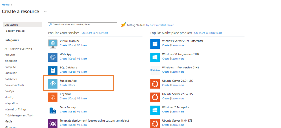
This brings us to the function creation screen, where we have to provide some configuration details before our function is created:

• Subscription: Azure subscription in which you want to deploy your Azure Function App
• Resource group: container that holds related resources for an Azure solution - these resources typically share the same development lifecycle, permissions and policies, ...
• Function App Name
• Runtime stack: Python
• Version: choose 3.9 (latest supported version) unless you have specific Python version dependencies.
• Region: choose the same region as other resource that you need to deploy e.g., blob storage, Cosmos DB, etc. ...
• Operating system: only Linux is supported
• Plan type: leave it to Consumption (Serverless) unless you have very specific requirements with regards to execution time limit higher than 10 minutes (see Azure functions scale and hosting - function app timeout duration for more details)

In the next configuration screens just leave the default options but do make sure that you link up an Application Insights resource to your Azure function.

Setup your development environment

Things to setup beforehand:

• Azure subscription
• Azure Functions Core Tools version 4.x
• Supported Python version (minimum Python 3.6  or a distro like Anaconda or Miniconda
• Visual Studio Code
• Python extension for Visual Studio Code
• Azure Functions extension for Visual Studio Code

Create your local Azure Function project in VS Code

Let's now see how you can create a local Azure Functions project in Python - open the Command Palette and choose Azure Functions: Create function. Next select Python, the Python interpreter to create a virtual environment, the template for the function (HTTP trigger) and the authorization level. Based on the provided information, Visual Studio Code will generate the different files in your project.

When you choose "HTTP trigger", it means that the function will activate when the function app receives a HTTP call. The name that you specified for the Function name (jopxtickerdata) will be used to create a new directory which contains three files:

• function.json - configuration file for our function
• sample.dat - sample data to test the function
• __init__.py  - main file with the code that our function runs

You can also add in your own Python code files (e.g. jopxlib.py) that you can use afterwards __init__.py , see Azure Functions Python developer guide - Import behavior for more details.

In the root directory of your project you will also see other files and folders:

• local.settings.json: stores app settings and connection strings when running locally
• requirements.txt: list of Python packages the system installs when publishing to Azure
• host.json: configuration options that affect all functions in a function app instance
• .venv:   folder which contains the Python virtual environment used by local development.

I slightly modified the standard generated HTTP trigger so that it accepts 2 query string parameters (name and startdate), added a reference to my own Python code (jopxlib) and called the writetickertoazblob function within the main function.

The code of  writetickertoazblob is quite simple - it will download data from Yahoo Finance in a dataframe and then save the dataframe to CSV and upload it to Azure Blob Storage. in Azure functons, application settings are exposed as environment variables during execution os.environ["AZURE_STORAGE_CONNECTION_STRING"] will read the application setting with name AZURE_STORAGE_CONNECTION_STRING

References:

• Quickstart: Create a function in Azure with Python Using Visual Studio Code
• Status of Python versions -  info on the Python language version support policy timeline
• Serverless Python Applications with Azure Functions - YouTube recording Build 2019
• An introduction to web scraping with Python and Azure Functions (YouTube)

Quick tip: troubleshooting Jupyter notebook not starting correctly

The other day my Jupyter notebooks did not start correctly from Anaconda navigator - luckily the Jupyter docs have a section  Jupyter - What to do when things go wrong. So I tried starting it from Anaconda prompt and it indeed gave me an exception that there was an invalid path in the Jupyter config file - to find out where to look for the config file check out Jupyter common directories and file locations

Quick tip: updating Anaconda with command prompt

 I recently started getting a popup for updating Anaconda Navigator on my Windows machine and I also received a warning when installing packages using the Anaconda prompt. I first started the update through the user interface but this update completely stalled and I had to do a hard reboot after almost 2 hours (when my patience ran out). Running the update using Anaconda prompt worked without problems - next time I will use this method first. If conda is installed on your machine, you can update it to the most recent version and patches using  conda update -n base -c defaults conda

Speaking engagements in coming months

With all Covid bans lifted and summer holidays well over, the conference season kicks off. 

I will be speaking at a couple of events in the coming weeks and months:

• Dataminds evening session Upcoming in-person event on September 29th organized by dataMinds.be at Inetum-Realdolmen offices in Kontich together with Benni De Jagere. First session a little bit off the beaten track for data professionals: #dataviz for investors. Second session: #PowerBI roadmap and #AMA by Benni.
• Collabdays Belgium 2022. Free community-driven event in Brussels, Belgium. Focus is Microsoft 365 with some Power Platform and Azure sprinkled on top. I am particularly excited to be speaking at this conference which was born out of the SharePoint Saturday conferences which I helped organize many years ago. I will be delivering Dataverse Deep Dive: watch out for sharks.
• Cloudbrew 2022. A two-day conference focusing on all things Azure on November 18-19 in Mechelen Belgium. I will be delivering Using Python and Azure Cloud for trading and investing

Using the yFinance Python package to download financial data from Yahoo Finance - part 2

In a previous post I showed how you can download ticker data from Yahoo Finance using the yFinance Python package.  I now updated the  Jupyter notebook code sample using YFinance to also show how you can retrieve additional information (sector, industry, trailing and forward earnings per share, etc...). The Ticker class in the yFinance library contains the info property which returns a dictionary object ( a collection of key-value pairs where each key is associated with a value) which allows you to access specific information about an asset.

Since I wanted to know how fast data retrieval would be I also include the %%time magic command . Wall clock time measures how much time has passed. CPU time is how many (milli)seconds the CPU was busy.

Yahoo Finance contains data about stocks, Exchange Traded Funds  (ETF), mutual funds and stock market indices - the information that you can retrieve for each of these differs, so it is safe to check in your code for the quoteType. Below example retrieves information about Apple stock, the iShares MSCI AWCI UCITS ETF (Acc) and a thematic mutual fund from KBC.

I also included a code snippet which shows how to retrieve this information for multiple assets and convert this into a Pandas dataframe.

Using the yFinance Python package to download financial data from Yahoo Finance

In a previous post I explained how you can retrieve data from Yahoo Finance using Python and Pandas Datareader - an alternative Python library for retrieving data from Yahoo Finance is yFinance maintained by Ran Aroussi. 

If you are using conda package manager, you will notice that you can not install yfinance using conda so you will need to revert to pip install yfinance. All documentation is available on yFinance  as well as on https://github.com/ranaroussi/yfinance but I also uploaded a  Jupyter notebook code sample on my Github - https://github.com/jorisp/tradingnotebooks/blob/master/yfinance_sample.ipynb

Using Python and Pandas Datareader to retrieve financial data - part 3: Yahoo Finance

Yahoo Finance is one of the most popular sources of free financial data. It does not only contain historical data but also financial statements, dividend information and calculated metrics like e.g. 50 and 200 day moving average, beta, etc ... Yahoo Finance does not have an officially supported API anymore but pandas-datareader  still allows you to access the data from Yahoo Finance in Python (other alternatives are yfinance and yahoo_fin).

This post is part of a series on using Pandas datareader to retrieve financial data:

• Using Python and Pandas Datareader to retrieve financial data - part 1: Federal Reserve Data (FRED)
• Using Python and Pandas Datareader to retrieve financial data - part 2: Fama & French library
• Using Python and Pandas Datareader to retrieve financial data - part 3: Yahoo Finance

In this post I have used version 0.10.0 of pandas-datareader  (released July 13, 2021) which is currently working with Yahoo Finance - previous versions of pandas-datareader had to be updated after Yahoo made some changes on the underlying API.

Warning: Accessing Yahoo Finance using Python libraries is quite brittle so don't try to built production trading systems using this data source.

Accessing the Yahoo Finance API using pandas-datareader is very simple as shown in the screenshot below but I would also recommend implementing a cache mechanism for your queries using the requests-cache Python library to avoid having your IP address being banned. The full source of this Jupyter notebook is available at https://github.com/jorisp/tradingnotebooks/blob/master/YahooFinancesingle.ipynb

References:

• Yahoo Finance API - A complete guide
• yfinance 
• yahoo_fin

Using Python and Pandas Datareader to retrieve financial data - part 2: Fama & French data library

This post is part of a series on using Pandas datareader to retrieve financial data:

• Using Python and Pandas Datareader to retrieve financial data - part 1: Federal Reserve Data (FRED)
• Using Python and Pandas Datareader to retrieve financial data - part 2: Fama & French library
• Using Python and Pandas Datareader to retrieve financial data - part 3: Yahoo Finance

In this post we will look at the datasets made available by Eugene Fama and Kenneth French. Eugene Fama and Kenneth French did a lot of research on which factors drive security returns. In 1993, they published the Three Factor Model (see article "Common risk factors in returns of stocks and bonds", Journal of Financial Economics 33, 1993), which showed that their factors (size of the firm, book-to-market values and excess return) capture a statistically significant fraction of the variation of stock returns. In 2014, Fama and French adapted their model to include five factors.  Fama won the Nobel Prize for Economics in 2013 for his research. Fama also published a number of papers on the Efficient Market Hypothesis and random walk theory.

Fama and French still publish the returns of various investment factors analyzed by them on their homepage on a regular basis.  You can download this data using the pandas_datareader library - you can take a look at the official documentation,  Fama-French Data (Ken French's Data library) to get started or take a look at the Jupyter notebook that I shared on Github https://github.com/jorisp/tradingnotebooks/blob/master/FAMA.ipynb

References:

• Fama/French forum ideas and observations from Fama and French
• How to use the Fama French model
• Fama-French 5-factor model: five major concerns
• In pursuit of the perfect portfolio: Eugene F. Fama (YouTube - MIT Laboratory for Financial Engineering )

Using Python and Pandas Datareader to retrieve financial data - part 1: Federal Reserve Data (FRED)

The pandas-datareader Python library covers a number of APIs with global fundamental macro- and industry data sources including the following (for a full list see  Pandas Datareader - data sources ):

• St. Louis FED (FRED): Federal Reserve data on the U.S. economy and financial markets
• Fama/French data library : market data on portfolios capturing returns on key risk factors like size, value, and momentum by industry
• Yahoo Finance : retrieve daily stock prices, historical corporate actions (dividends and stock splits) from Yahoo Finance 
• World Bank: global database with economic/social indicators and demographics.

This post is part of a series on using Pandas datareader to retrieve financial data:

• Using Python and Pandas Datareader to retrieve financial data - part 1: Federal Reserve Data (FRED)
• Using Python and Pandas Datareader to retrieve financial data - part2: Fama & French library
• Using Python and Pandas Datareader to retrieve financial data - part 3: Yahoo Finance

In this post I will focus on retrieving data from FRED using pandas-datareader.  Federal Reserve Economic Data (FRED) - https://fred.stlouisfed.org/  is a database maintained by the Federal Reserve Bank of St. Louis. It has more than 800.000 data time series covering categories such as Economic growth & employment, monetary & fiscal policy, demographics, industries, commodity prices at different frequencies (daily, monthly, annual).  One of the interesting time series you can find here are 3-month Treasury Bill Secondary Market rate (TB3MS) or 1-year US Treasury bills which are used a proxy for the risk free rate in financial modeling. 

There is however some missing data on the TB1YR - so I will be using the TB3MS (3 Month) in my next example. You will notice that all time series are identified by a short abbreviation that you can find by searching on the FRED website.

Full source code is available at https://github.com/jorisp/tradingnotebooks/blob/master/FRED.ipynb 

References:

• FRED API: get US economic data which drives the real estate market
• Pandas-datareader python library